Problem Definition

Let us denote asset weights by ⃗. We denote the function which, given the asset weight vector , computes the percent contribution to risk from each of the ⃗K  factors. When the risk metric is the volatility of the portfolio, then f(x) takes the following form:

(1)

where ⊙ is the element-wise dot product between two vectors, is the vector of exposures for the portfolio, is the factor covariance matrix. The objective function that we seek to minimize is:

(2)

where is the original asset allocation of the portfolio, represents the  norm, and represents the norm. The  norm penalty term seeks to minimize the size of changes between the original asset allocation and the optimal allocation, and  norm helps to reduce the number of changes between the original allocation and the optimal allocation.

1) While in the simplest case, the risk measure used is the volatility, we can envision the use of other metrics such as CVaR or Expected Shortfall. Then the function f(x) computes the percentage contribution to the CVaR or Expected Shortfall.

2) The true norm to minimize the number of changes between the optimal portfolio and the original portfolio would be the  norm, which is non-convex. Hence, we use its closest convex cousin — the  norm — to impose the fewest trades constraint.

3) Since the assets in the target portfolio and the client’s original portfolio can be different, the function f(x) is computed on the expanded client portfolio. Let the set {x} denote the set of assets in the client’s original portfolio and the set {xtarget} denote the set of assets in the target.
Then the portfolio to be rebalanced is the set of assets {xrebalance} = {x} ∪ {xtarget}. The additional assets in this expanded set are set with an initial asset weight of 0.

Adding Client Constraints

Client constraints are the general set of asset allocation preferences that need to be accounted for when performing a rebalance. Broadly, these can be classified into IPS bounds and asset-specific restrictions. 

IPS Bounds 

An IPS or Investment Policy Statement is a document that serves to define the objectives for a client portfolio. In particular, an IPS defines the time-horizon and investment goals for the portfolio. Along with more general details, it also defines client-specified ranges for certain asset classes. A simple example could be that the client only wants between 20 and 30% of their portfolio in Equities and an even smaller amount between 2-5% in alternatives.

These IPS bounds can be taken into account as extra constraints to the original objective function defined in Equation 1 above. We do that as follows.

Let {1 ... N} be the indices of the expanded set of assets {xrebalance} . Then forM asset-classes,
we haveM partitions of {1 ... N} noted such that . The IPS bounds for each of the M asset classes can then be written as:

(3) (4) 

where are the lower bounds and are the upper bounds for each of the asset classes.

Restrictions 

Client specified restrictions are restrictions on buying/selling of certain securities within the portfolio. These restrictions could be imposed for many reasons. For instance, an executive in a big tech firm might not wish to sell their equity stake in their company. Or there could be legacy holdings that a client might wish to keep.

Irrespective of the reason for the restrictions, the rebalance should account for these. These restrictions can be accommodated as extra constraints on the objective function defined in (2) above.

These restrictions can be of multiple types. Let the asset index be denoted by I where I can have more than one element since the same asset can be present in more than one account. Then we have:

1) Do not buy: i.e. the final allocation can’t be more than the original allocation for that asset.

2) Do not sell: i.e. the final allocation can’t be less than the original allocation for that asset.

3) Do not trade: i.e. the final allocation must be equal to the original allocation for that asset.

4) Exclude: This restriction implies that for the asset in consideration, we must exclude it from the rebalance. Thus the set of assets over which the objective function in (2) is defined becomes  where - stands for set exclusion.

As an extension of asset-specific restrictions, we can also specify account-level restrictions. In this case, we drop the sum over the accounts, and the index I then stands for the index of assets for the specified account.

Cash 

Cash and cash holdings need to be handled separately since a client might want to keep a certain weighting of their portfolio in cash. Within the Fabric application, we will consider cash as a “free” source of funds to be deployed in order to achieve the rebalance objective as closely as possible. By default, all cash should be deployed. However, if the advisor over-rides this default then they must specify the level of cash to be left within the portfolio. This specific case of cash can then be accounted for as an extra constraint to the objective function in (2).

Let the index of cash holdings be denoted as C, where once again cash holdings can be present in multiple accounts. Then the constraints are of the form

   (5)

Note that we only allow the deployment of cash within guided rebalance. Raising cash holdings
by selling assets is not within the scope of guided rebalance.

Complete Formulation 

Guided rebalance is then an optimization problem with the following form:

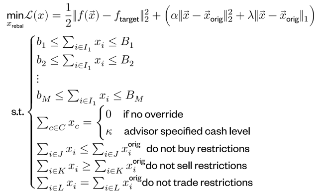
The optimization problem above has an objective function that can be written as a sum of squares. The function f(x) as defined in (1) is a non-linear function of the asset weight vector . Thus, the op- ⃗x timization problem falls in the realm of non-linear least squares programming. Many algorithms exist to solve such problems. Within the Fabric analytics engine, we use Sequential Least Squares QP (SLSQP) Algorithm to minimize the objective function subject to the IPS, account, cash, and trading restrictions.